This explainer begins by contrasting supervised and unsupervised learning algorithms, but they're not in competition. The key takeaway for aspiring data scientists is that the choice between a supervised or unsupervised learning approach hinges on the specific task.
Frequently in a machine learning workflow, from raw data to the deployed model, both unsupervised and supervised learning models are utilised together.
Supervised Learning: Learning from labeled data
So supervised learning is about learning from labeled data. We have inputs and associated outputs or target variables and we want to build an algorithm that mimics this process, for which it performs well on training data, but most importantly on unseen data. This idea of building a machine that can predict outcomes in new unseen situations or configurations is central to the concept of generalisation.
There are two principal supervised machine learning techniques: regression and classification algorithms. It's not that one is better than the other; rather, they are different types of supervised learning algorithms for different types of data. It all comes down to what the output data or variable looks like.
If the data is a class or a label, then the supervised learning algorithm is called a classification algorithm. Whilst if the output of the prediction is a number - aka a real or continuous value (e.g. temperature, stock price) then the supervised learning task is called regression.

Figure 1. Examples of supervised learning task (LEFT) a machine learns how to identify a cat from labeled data of pictures of cats and dogs. supervised classification task. on the right is a response surface or curve fitting, an example of supervised regression.
A random forest, k nearest neighbour, deep neural network, support vector machine, linear regression, or logistic regression are all good examples of supervised learning algorithms.
The performance of supervised learning algorithms is typically easy to access, an algorithm that accurately predicts the output variables for unseen inputs can be computed and benchmarked against other approaches.
Let's take a bit of a deep dive and look at three supervised learning algorithms
k Nearest Neighbour (aka kNN)
kNN is a really nice and conceptually simple supervised learning algorithm. Which can be used for both regression and classification tasks. In this little toy example, we are going to look at a classification problem.
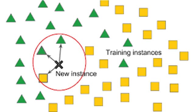
Figure 2. Simple toy representation of KNN
In this picture what we have is a 2D space which represents the space of possible. data. For different inputs (locations in this space) each sample has been assigned a label. For some green triangles, for others yellow squares.
The method proceeds in a really simple way. First for a new location (not seen by the data before) - here marked X "New Instance", we look for the k (here k = 3) nearest neighbours to this point. We then make a prediction on the class label, by taking a majority vote, dependent on the class labels of the neighbours. Here in this pictured toy example, we see that 2 of the 3 neighbours are green, and with that, the supervised machine learning algorithm predicts a "green triangle" label for the previously unseen data.
In general, kNN is a really simple algorithm and a great starter algorithm to learn on your machine learning journey!
Curve Fitting or Response Surfaces
Curve fitting is often not seen as a machine learning algorithm by itself. However, it is at the core of supervised machine learning models. For a response surface with simple constructions, such as the composition of polynomials, these models are often easy to train. They are naturally suited to regression-based tasks, in which they predict output data that is a real or continuous value. However, they can also be extended to classification algorithms, for example, by using logistic regression.
Deep Neural Networks
Deep neural networks (DNNs) are a type of machine learning model. DNNs are based on the concept of artificial neurons — connected layers of nodes that mimic how nerve cells in the brain interact and process information. The connections between these nodes can be “trained” using a machine learning workflow.
The training process uses known inputs and outputs to adjust the weights of connections between nodes so that when presented with unseen data, the model can make accurate predictions. DNNs enable computers to learn complex patterns from data and make decisions based on these learned patterns. As such, DNNs are widely used in many areas of AI research.
Traditionally deep neural networks are used for supervised machine learning tasks, however, there are clear exceptions to the rule. Autoencoders are a widely used unsupervised learning model, whilst reinforcement learning is also dominated by DNNs. DNNs play a central role in modern machine learning.
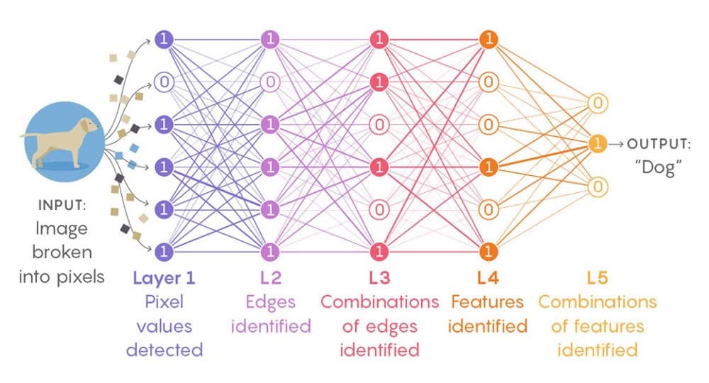
Figure 3. Diagram shows a visual demonstration of a deep neural network, applied to an image recognition problem of images, with our classic problem 'is it a cat?'
Unsupervised Learning: Finding Hidden Patterns
Unlike supervised learning, unsupervised learning uses unlabeled data points, and therefore only uses input data. Its purpose is to extract hidden patterns or inherent structure, which is often found in large data sets. By drawing out these patterns, unsupervised machine learning can assist in bringing new insights from data, or help fashion data representations that are more efficient and suitable for subsequently building supervised approaches.
Just like supervised learning, unsupervised learning algorithms are split into two primary classes.
Unsupervised learning clustering algorithms.
Clustering algorithms are a set approach that takes unlabeled data and collects them into groups, with the aim that samples within each group are "alike". This allows data scientists to draw insights from the data sets, build better models (potentially by considering each cluster in turn) or can be used to guide sample collection - see semi-supervised learning.
There are various clustering algorithms, the one we briefly consider here is k-means. In k means, data is placed into the cluster whose centroid (average point) is closest. Here the k refers to the number of clusters and must be determined as part of the tuning process. It is one of the simplified unsupervised learning models and is a great one to know.
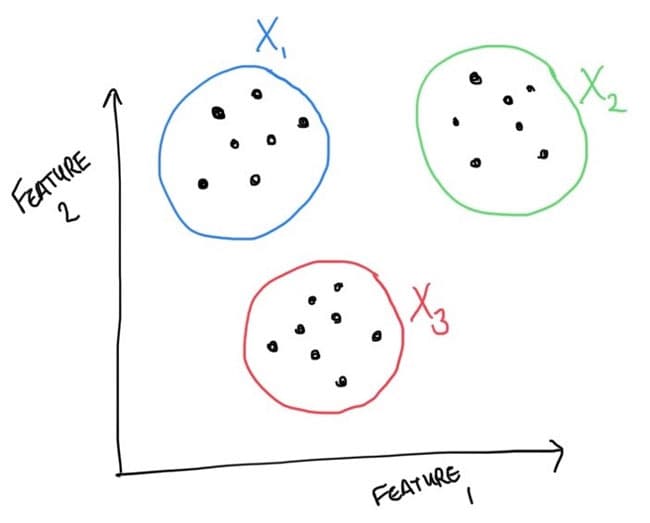
Figure 4. Representation of k-means. splitting input data into three independent clusters. input data is assigned to the cluster whose centroid is close to the data point.
Unsupervised Learning for Dimensionality Reduction
So a key challenge in machine learning is the curse of dimensionality - as the size or scale of the input data (the dimension) increases then the data requirements of the algorithms grow exponentially. Therefore a key component of building machine learning models is design methods, which reduce the dimension of the input data, so what is retained is reduced to the important or salient features which are sufficient to still make good predictions or decisions.
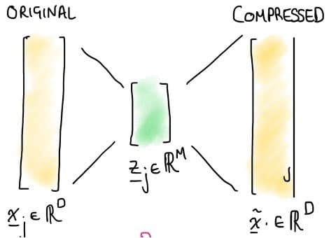
Figure 5. Demonstration of the principle of dimension reduction, the simplification of reduction of input data into a salient feature space (shown here in the center in green). This reduced dimension allows much more efficient machine learning models to be built.
There are various methods for dimension reduction for feature selection, for example, some can be done as part of a supervised learning model (e.g. LASSO - look it up). Here we have a quick peek at Principle Component Analysis (aka PCA).
Principal Component Analysis (aka PCA)
Let's first look at a simple picture and then say how it relates to PCA.
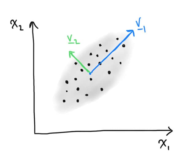
Figure 6. Visualisation of principal components in a simple 2d synthetic data set.
What we see here is the principle component of a data set in 2-dimension. The principle components are a set of order vectors here denoted and in this example. The first direction (or vector) in the data aligns with the direction which drives the most variance in the data, the second direction here denoted is orthogonal (at right angles) to the first direction with the second largest variability in the data.
As we have only shown a 2D example, there are only two principal directions. The idea here is that if we want to reduce the model to a single dimension, we project (or collapse into) a single direction. Then the first principle component () retains the most variability in our data, therefore in an unsupervised setting (without knowing anything about our task) is a good way to reduce the dimension of data.
Importantly the PCA automatically gives the relative importance of each of the principle components, this is a measure called explained variance. With this, users can quantify how much of the "variance" in the data set is lost if a truncation to a smaller dimensional space is used.
Semi-supervised learning
Semi-supervised learning is a type of Machine Learning workflow that uses both labeled and unlabeled data for training. It takes advantage of the large amounts of relatively inexpensive unlabeled data available, as well as the accuracy of models trained on labeled data, in order to improve the overall performance of the model.
By combining these two datasets, semi-supervised learning is able to provide accurate predictions with less data than traditional supervised learning methods. Semi-supervised learning can be used in a wide variety of applications, from text classification and image recognition to anomaly detection and natural language processing.
In addition, it has been successfully applied to deep neural networks for improved accuracy and speed. Ultimately, semi-supervised learning offers the potential for higher accuracy and faster training times than traditional supervised learning on similarly sized datasets. This makes it a powerful tool for data scientists who need to quickly create accurate models with limited resources.
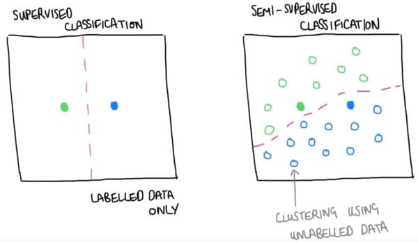
Figure 7. Demonstrates the core principle of semi-supervised learning. large amounts of unlabelled data are used to supplement limited labelled training data to build more data-efficient methods.
Let's look at it in a bit more detail, through a very simple pictorial example in which we seek to classify data. On the left, we see a labeled dataset, with labels from two different classes. In a purely supervised learning set, the best we can do is separate the input space, by placing a simple decision boundary halfway between each sample. Can we do better?
Suppose we also have lots of unlabelled data, how can we use it to make a better classification model? The idea in semi-supervised learning is shown on the right. We cluster unlabelled data with the cluster data, then by proxy (in terms of cluster) assign the same label (a pseudo-label) to the unlabelled examples. With this unlabelled data, we can now build a richer decision boundary, which we hope addresses the limited labelled data challenges, demonstrated in the setup shown on the left.
Reinforcement Learning
Last but not least we branch out and look at a different type of learning which is increasingly getting more and more traction.
As an aside, I write up this introductory explainer article on the day I met Richard Sutton whilst attending CDL super session in Toronto. If you don't know his work, then look him up. If you want an accessible route into the details of Reinforcement Learning, his book, Sutton & Barto and the associated material, is great!
Let me first tell you about my favourite application of reinforcement learning.
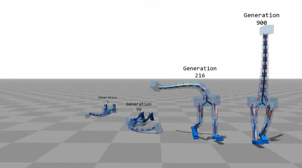
Figure 8. My favourite example of RL
So what are you looking at? You are looking at a new creature, a sort of two-legged giraffe. In this study, reinforcement learning methods are used to iteratively work out how the animal should control their muscles in a coordinated way to move forward whilst remaining stable and upright. The learning algorithm learns by experience, learning a "policy" - a strategy by which to act given observations of an environment and a sequence of positive and negative feedback. Over time, here 900 generations of policies, the animal learns how to effectively walk.
In a general setting machine learning, learns by reinforcing behaviour which leads to good outcomes. It more strongly aligns with how humans (particularly children) learn to do new tasks without directly supervised demonstration (although this can accelerate learning).
The reinforcement learning process involves a loop between an 'Agent' and the 'Environment' within which it operates. This loop consists of three cyclical components. First, the 'State,' which is the observable condition of the environment from the agent's perspective. Next, the 'Action,' which represents the choices the agent can make or the actions it takes. Finally, the 'Reward,' which is the feedback or outcome the agent receives based on its action.
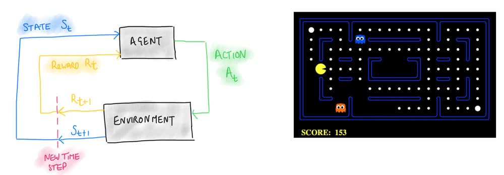
Figure 9. The general setup of a single agent reinforcement learning group. pacman a playground for building and testing new RL methods.
Innovation in Reinforcement Learning has primarily revolved around games. Not only are games enjoyable, but their rules, actions, and configurations are also well-defined, making them a productive platform for exploring new methods.
As Richard Sutton showed, we could write a book on these methods (and more!) Here we touch on the two primary approaches to reinforcement learning. Just like supervised learning and unsupervised learning, it is not either/or, and often the good approaches use them in combination.
Value-Based Methods
The general principle around value-based methods is for an agent to take actions that move the system to the highest expected realizable value. The machine learning algorithm works by learning a model which maps from a "State" and "Action" pair to an expected value, a number.
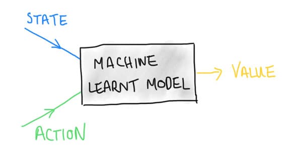
Figure 10. Value-based learning seeks to understand the value of taking an action in a particular observed state.
The value of taking an action, when in a state is calculated by experience. What is the expected future reward outcome if an action is made? We often follow this approach as humans. Here is a simple example in the final step of the noughts and crosses game.
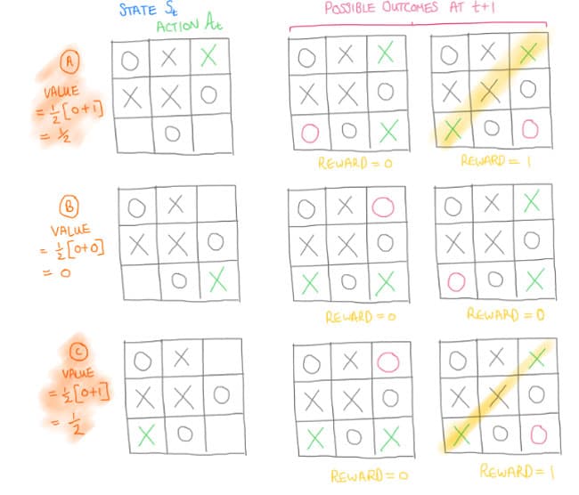
Figure 11. Simple example of the final move of noughts and crosses to demo value-based learning.
In this case, we look at the decision of the one but last move of a "cross". The approach tries to assign a value to each of the actions, given a current state. We see that two actions lead to an equal possible chance of a win, whereas one move eliminates the chance of a win completely. This makes our action clear in this simple setting.
Value-based learning methods extend these principles to much more complex situations. To take a start in this space, look up Q-learning.
Policy Based Methods
A policy is a mapping from "State" to "Action", what action should I do in a given state. Policies are learned to not minimise a loss function as in supervised learning, but instead to maximise the expected reward. Therefore many machine learning tools, as for Value-based learning, can be used in policy base RL methods; and often the most popular are deep neural networks (see above).
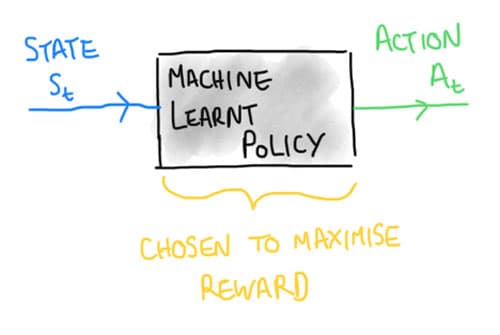
Figure 12. Policy based methods are about understanding the mapping from a state to action for an agent.
Concluding Points
We take a fly-by tour of the core principles or ideas behind supervised and unsupervised learning. In no way is this a complete thesis, but lays the high-level landscape, so you can understand the difference in fundamental tasks that machine learning models can carry out, and what you might do with labeled and unlabeled datasets in your business or studies.
From this, we then take one step further and show that machine learning is not just this simple divide between supervised vs unsupervised learning, but of course, is more complex. This includes hybrid methods, called semi-supervised learning; which bring together for particular settings of a data set.
Secondly, we take a quick look at reinforcement learning, a field of machine learning where algorithms learn through experience; an exciting "new" area which is getting significant momentum in building new systems which display "intelligence" in operating or controlling complex tasks.