K - Nearest Neighbours - Your first supervised Learning Algorithm
k-Nearest neighbours (kNN) is a simple non-parametric, supervised learning algorithm in machine learning.
In this explainer, we will:
- Explain the basic idea behind kNN
- Unpack what we mean by non-parametric and supervised learning.
- Introduce a simple example to explain the intuition behind KNN.
- Understanding a more general concept of "distance”.
- Understand what the 'k' stands for in kNN and how you might choose an appropriate value.
The basics: kNN as a non-parametric, supervised learning algorithm.
Firstly, kNN is a supervised learning algorithm, this means that we have labelled data. For this discussion, we will call our input data
and our associated target data
In this dataset, we have pairs of input values and target values so that .
The challenge set out in supervised learning is, given a new unseen input , can we make a prediction of the target value .
In kNN, the idea is very simple; we find the nearest points to which belong to our training data set . We then use the average target values of those selected points as our prediction for the new point .
kNN is described as a non-parametric method. I remember being told this at first and thinking this is odd since it seems like , the number of neighbours I choose to average over, is a parameter and I have to select it. More on in a minute. But what non-parametric means is that there are no underlying assumptions (parameterisations) of the data. kNN is therefore particularly effective if
- If you have lots of data and in some sense have good "coverage" of your possible input space.
- You have a poor understanding of the underlying distribution of your data; the data is easily interpretable and/or there are complex non-linear relations in your data which cannot be easily parameterised.
We will discuss how you pick your in a minute but first let's look at a picture to get a better idea of what we mean.
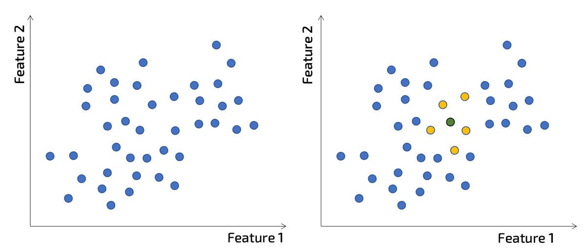
Here we have a training data set, which represented by blue dots (in the left figure).
We then want to make a prediction for input located at the green dot (right picture). In this example we see that the yellows are the nearest neighbours.
Now a nice thing about kNN is we can use it for both regression and classification task. So let's look how this might work
Regression
There are two simple variations of kNN - these are average vs weighted average. These are two variations of how predictions are made. The simple version is that the known target values for the k nearest neighbours are simply averaged. Each point contributes equally.
So here in this toy example above, the value at the green point is equal average of it's 5 neighbours. If the value at the 5 neigbours are
An alternative is we weight contributions, where more contributions are made by those training data points which are "closer" to.
So if we say denotes the distance between the th closest neighbour and the new point, we can define the weight for the th neighbour
so then the preditions is made as follows
When you have a densely populated dataset, then the distance from an unseen point with it's neighbours will be almost equal. Hence the difference between these two approaches diminishes as a fuction of amount of data and k (number of nearest neighbours).
In general I would default to the weight distance, whilst a bit more to calculate, you will see that the packages that implement kNN do this for you, and the extra costs of including the weights is minimal.
Classification
Classification is nice and easy, once you have found your nearest neighbours, you can do majority voting. What do we mean by this. So you will have got labels from your the neighnest neighbours. You tally up the number of each of the labels in that group, and the predicts is the one with the most "votes" for that label.
In the case where you had equal numbers of votes for a label, you could randomly sample, from the labels with equal weights.
There are more complex versions. Just like the regression task, the vote could be weighted by the distance from the point. This would work in a similar way. The "vote" count for each label would be the sum of the weights of all neighbours with the sample label. Then majority voting is applied in the same way.
The good, the bad and the ugly.
It is clear to see that there are some advantages and disadvantges of kNN.
| Advantages | Disadvantages |
|---|---|
| Very Simple. Easy to implement and easy to understand. Therefore as long as your data set isn't huge, then worth a try, before going more complex. | A simple implementation of kNN would be very slow for large data sets. This is because a simple implementation requires calculating the distance between each pair of samples. |
| It has a level of identifiability to it, in that the algorithm points to examples in a existing data set which inform the predicted value. These training points can be natural interograted. | The approach requires significant about of data, to make good predictions there needs to sufficient data, how much is problem dependent since it really depends how smooth the target value is being predicted. |
What do we mean by distance?
Central to the knn algorithm is to find the distance between the new points and each of the existing training points. For a bit of notation we might write .
In general when we say distance, we think of physical distance. Yet that only really makes sense when we are comparing physical coordinates. For example how close is the label 'cat' to 'dog' for example, our traditional understand. In mathematics this introduces a whole feel of understanding distances - which are called 'metrics' and importand concept in machine learning is this idea of 'metric learning' - where by you find the best way to measure distance to give you the best model. We will talk about a simple example of this in a minute.
So here are the three most common measures of distance
-
Euclidean Distance. This is our traditional measure of distance between two points and is calculated
-
Manhattan Distance: This is the distance between real vectors using the sum of their absolute difference, and so
-
Hamming Distance, which is used for discrete categorical variables. If two variables are the same the distance is zero, else 1.
How to choose k?
So the final piece of the jigsaw is how to choose the valye of k. A small value of k means that the algorithm is more sensitive to outliters and noise in the data, whilst a larger value of k, has a smoothing effect averaging noise out of a large number of data points, but with that reducing accuracy. The better value (not I don't say optimal) are a compromise.
The optimal value k is often determined through cross-valuidation (their others e.g. the elbow methods).
So how does cross-validation work?
The idea with cross-validation is to estimate the expected error - which we will call . This can be done by dropping out a sample from the training set, and then use kNN to predict the target value which . The process is the repeated over all samples times, and we can then take the mean (or expected) error.
Note that we introduce a subscript to which denotes the choice in value of .
If the data set is large often the error is approximated by randomly sample only a few samples, rather than estimating the error over the whole data set.
We can repeat this process of different values of k, so we would typically get a plot like the following (which I have knicked from the full example below).
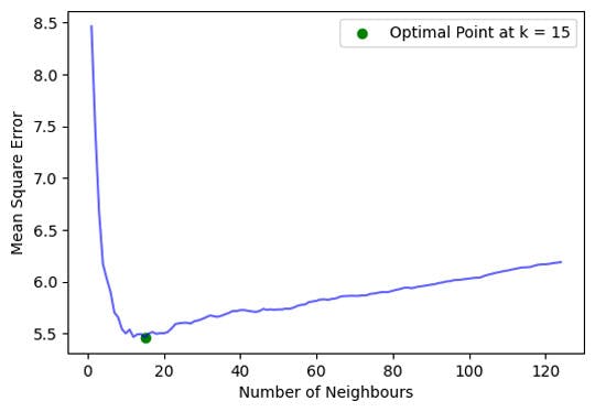
What we see is for a very low value of k (suppose ), the model overfits on the training data, which leads to a high error rate on the validation set. On the other hand, for a high value of k, the model performs poorly underfitting. If you observe closely, the validation error curve reaches a minima at a value of k = 15. This value of k is the optimum value of the model (but will clearly vary for different datasets or test/train splits of the same data set).
In the example below we can use a simple grid search to find a good value of k, which we show how to apply in the example below.
Conclusions
One of the main advantages of the kNN algorithm is its simplicity. The algorithm is easy to implement and understand, and it does not require any complex mathematical operations. Additionally, it is a lazy learning algorithm, which means that it does not require any training data to be stored in memory. Instead, the algorithm only needs to store the training data and then use it to make predictions on new data.
However, there are also some limitations to the KNN algorithm. The algorithm can be computationally expensive when dealing with large datasets, as it needs to calculate the distance between the test point and all the points in the training set. Additionally, the algorithm can be sensitive to the scale of the features, and it may not perform well when dealing with high-dimensional data.