In this explainer we are going to look at a first example of using k Nearest Neighbour. This will give you a basic idea of how kNN is used and also a simple way to determine a good value of .
Add Libraries
As normal we start by adding some standard libraries for various functions we will use generally
import pandas as pd
import numpy as np
import matplotlib.pyplot as plt
A dataset of sea snails!
Ok so important stuff, can we predict the age (equivalent to number of rings) of a sea shell based on various simple measurements.
Let us first download the dataset and get moving.
url = (
    "https://archive.ics.uci.edu/ml/machine-learning-databases"
    "/abalone/abalone.data"
)
abalone = pd.read_csv(url, header = None)

abalone.columns = [
    'Sex',
    'Length',
    'Diameter',
    'Height',
    'Whole weight',
    'Shucked weight',
    'Viscera weight',
    'Shell weight',
    'Rings',
]

abalone = abalone.drop("Sex", axis = 1)
We dropped "Sex" as it is a categorical measurement, where all others are simple numbers. By dropping it, it makes life easier!
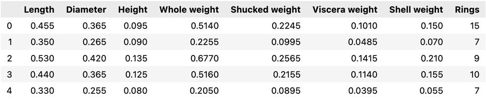
Ok, so let's look at our data
abalone.head()
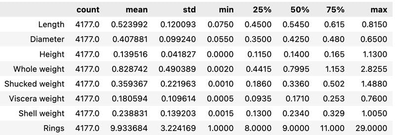
abalone.describe().T
X = abalone.drop("Rings", axis = 1)
y = abalone["Rings"]
We first want to rescale our data, we do this using an inbuilt frunction in sklearn. This transforms all variables to range of 0 to 1. It is vital in many ML algorithms, otherwise the inputs and their contribution to predictions are no handled fairly.
from sklearn.preprocessing import scale

X_scaled = scale(X)
Validation : Train / Test Split
So we are going to want to train our model, and then test it against held out data. Here we again use sklearn's inbuild functions, holding out 20% of the data for testing.
from sklearn.model_selection import train_test_split

X_train, X_test, y_train, y_test = train_test_split(X_scaled, y, train_size=0.2, random_state=42)
Fitting a Model
Now we are are in shape to fit a model. First we do this for a single given value, 10.
from sklearn.neighbors import KNeighborsRegressor
from sklearn.metrics import mean_squared_error

k = 10

knn_model = KNeighborsRegressor(n_neighbors=k).fit(X_train, y_train)

y_pred = knn_model.predict(X_test)

rmse = np.sqrt(mean_squared_error(y_test, y_pred))

print(rmse)
We see here the average root mean squared error is rings / years out.
So let's look at a validation plot over the whole of the testing set and see how we did.
import matplotlib.pyplot as plt

plt.figure(figsize=(6,4))
plt.scatter(y_pred, y_test, c='cornflowerblue', alpha = 0.1)

perfect_line = np.linspace(3,23,2)

plt.plot(perfect_line, perfect_line, '-k', alpha=0.6)

plt.title('Model Validation for k = 10')
plt.xlim([2,19])
plt.xlabel("Predicted")
plt.ylabel("True")
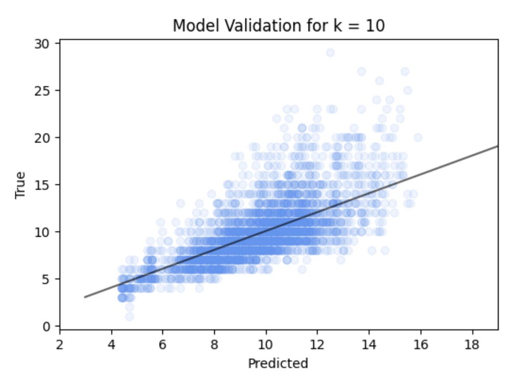
You will note some banding in this, this is because the number of rings is an interger number rather, than a continous number. Hence in this case a kNN classifier might yield better results, but we wont worry here as we are primarily looking at the general principles.
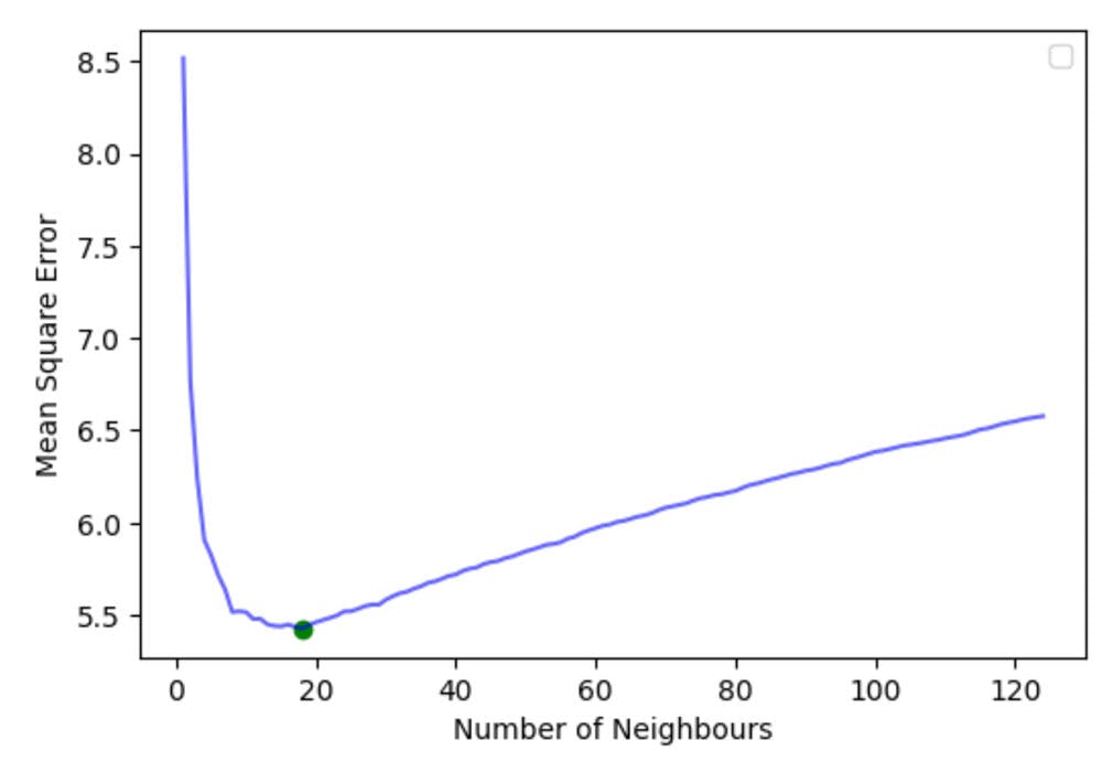
Choosing
So now we have built the model for a single value of , how do we explore the optimal value of ?
We now build models for all values of from all the way up to
k = np.arange(1,125, 1)

mse = []

for i, n_neigh in enumerate(k):

    knn_model = KNeighborsRegressor(n_neighbors=n_neigh).fit(X_train, y_train)

    y_pred = knn_model.predict(X_test)

    mse.append(mean_squared_error(y_test, y_pred))

optimal_k = k[np.argmin(mse)]

print(optimal_k)
The optimal is in this study.
Let us also plot out all the others.
plt.figure(figsize=(6,4))
plt.plot(k, mse, '-b', alpha = 0.6)
plt.scatter(optimal_k, np.min(mse), c='g')
plt.xlabel('Number of Neighbours')
plt.ylabel('Mean Square Error')
plt.legend()