We've chewed over the theory. Now let's see how this technique may be applied to a visual regression problem. Let's begin by generating some data.

RANDOM_SEED = 31
NOISE = 2
SCALE = 20

# Define the ground truth function
x = np.linspace(0, SCALE, 101)
y_true = 1.5 * (x -7 + 2*np.sin(x) + np.sin(2*x))

# Generate data skewed with noise
ep = NOISE * np.random.normal(size=(len(x),))
y = y_true + ep

# Columns
x = x[:, np.newaxis]
y = y[:, np.newaxis]

Here we consider the data-generating (ground truth) function

which is skewed, as $y(x) + \varepsilon$, with some normally distributed noise $\varepsilon \sim \mathcal{N}(0, 2)$. To see this data, let's fit a linear regression through the data points and plot the results.

from sklearn.linear_model import LinearRegression

linear_model = LinearRegression()
linear_model.fit(x, y)

print('Score: ', linear_model.score(x, y))
print('Coeff: ', linear_model.coef_)
print('Intercept: ', linear_model.intercept_)

x_test = np.linspace(0, SCALE, 1001)
x_test = x_test[:, np.newaxis]
y_pred = linear_model.predict(x_test)
y_gt = 1.5 * (x_test -7 + 2*np.sin(x_test) + np.sin(2*x_test))

scat = plt.scatter(x, y, marker='.')
line, = plt.plot(x_test, y_pred, 'g', linewidth=2)
true, = plt.plot(x_test, y_gt, '--r')
plt.legend([scat, line, true], ['Data', 'Prediction', 'Ground Truth'])

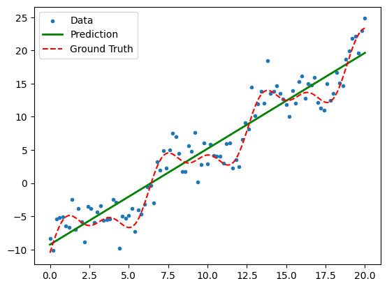
The linear fit produces a coefficient of determination (the R^2 value) of 0.90. Not bad, but given the non-linear form of the ground truth function, we have a strong prior belief that the model has not captured all of the features.

Now let us try a variety of kernel models to detect these features.

from sklearn.kernel_ridge import KernelRidge

# Polynomial kernel
krr_poly_model = KernelRidge(kernel='polynomial', degree=5)
krr_poly_model.fit(x, y)

# Radial Basis Function kernel
krr_rbf_model = KernelRidge(kernel='rbf')
krr_rbf_model.fit(x, y)

# Laplacian kernel
krr_laplacian_model = KernelRidge(kernel='laplacian', gamma=1/SCALE)
krr_laplacian_model.fit(x, y)

# Linear kernel
krr_linear_model = KernelRidge(kernel='linear')
krr_linear_model.fit(x, y)

# Test points
x_test = np.linspace(0, SCALE, 1001)
x_test = x_test[:, np.newaxis]

# Predictions
y_poly = krr_poly_model.predict(x_test)
y_rbf = krr_rbf_model.predict(x_test)
y_laplacian = krr_laplacian_model.predict(x_test)
y_linear = krr_linear_model.predict(x_test)

# Ground truth
y_gt = 1.5 * (x_test -7 + 2*np.sin(x_test) + np.sin(2*x_test))

# Plot results
fx, ax = plt.subplots(2, 2, figsize=(10, 10))

# Linear kernel
scat = ax[0, 0].scatter(x, y, marker='.')
line, = ax[0, 0].plot(x_test, y_linear, 'g', linewidth=2)
true, = ax[0, 0].plot(x_test, y_gt, '--r')
ax[0, 0].legend([scat, line, true], ['Data', 'Prediction', 'Ground Truth'])
ax[0, 0].set_title('Linear Kernel')

# Polynomial kernel
scat = ax[0, 1].scatter(x, y, marker='.')
line, = ax[0, 1].plot(x_test, y_poly, 'g', linewidth=2)
true, = ax[0, 1].plot(x_test, y_gt, '--r')
ax[0, 1].legend([scat, line, true], ['Data', 'Prediction', 'Ground Truth'])
ax[0, 1].set_title('Degree 5 Polynomial Kernel')


# Laplacian kernel
scat = ax[1, 0].scatter(x, y, marker='.')
line, = ax[1, 0].plot(x_test, y_laplacian, 'g', linewidth=2)
true, = ax[1, 0].plot(x_test, y_gt, '--r')
ax[1, 0].legend([scat, line, true], ['Data', 'Prediction', 'Ground Truth'])
ax[1, 0].set_title('Laplacian Kernel')

# RBF kernel
scat = ax[1, 1].scatter(x, y, marker='.')
line, = ax[1, 1].plot(x_test, y_rbf, 'g', linewidth=2)
true, = ax[1, 1].plot(x_test, y_gt, '--r')
ax[1, 1].legend([scat, line, true], ['Data', 'Prediction', 'Ground Truth'])
ax[1, 1].set_title('Radial Basis Function Kernel')

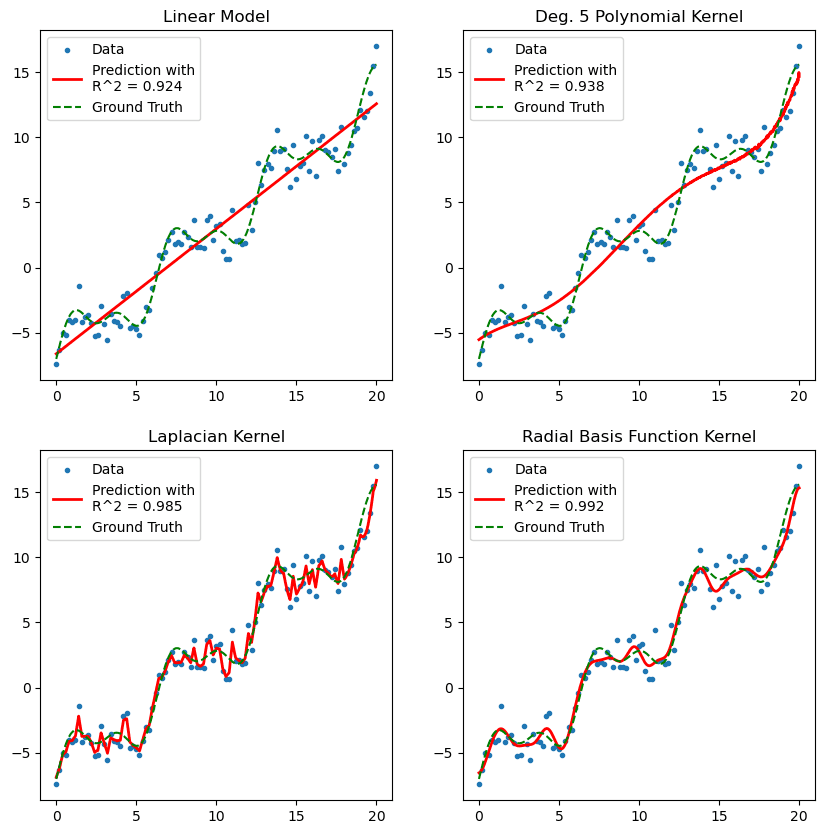
A few observations:

• The linear kernel under performs compared to our first linear model, as there is no built-in intercept.
• The degree-5 polynomial is constrained by dimension and therefore not expressive enough to capture the mixed periodicity in our ground truth data.
• The Laplacian kernel, whilst allowing an infinity dimensional feature representation, penalises higher order features.
• In practice, you shall most likely be turning to the Radial Basis Function (RBF), or Gaussian kernel, which here captures different scales of periodicity in the data trend.