- Three key types of kernel function:
- Polynomial kernels
- Squared-exponential kernels
- Laplacian kernels
- The effects of varying hyperparameters alters the prediction
- Kernel interpretation of the the motivating example projecting into 3D
Constructing kernels can be close an art form. A very important art form when it comes to understanding trends in data.
The ground zero example is the kernel formed by the inner product of the original data features . Other kernels may be found through sums, products, positive multiples of existing kernels. Three commonly used prototypes are:
- ; a polynomial kernel with constant and degree .
- ; the squared-exponential kernel, with 'inverse length-scale' .
- ; the Laplacian kernel, based on the taxi-cab norm .
In this video we shall explore how the various hyperparameters impact the prediction, and how the different choices of kernel can improve model fitting.
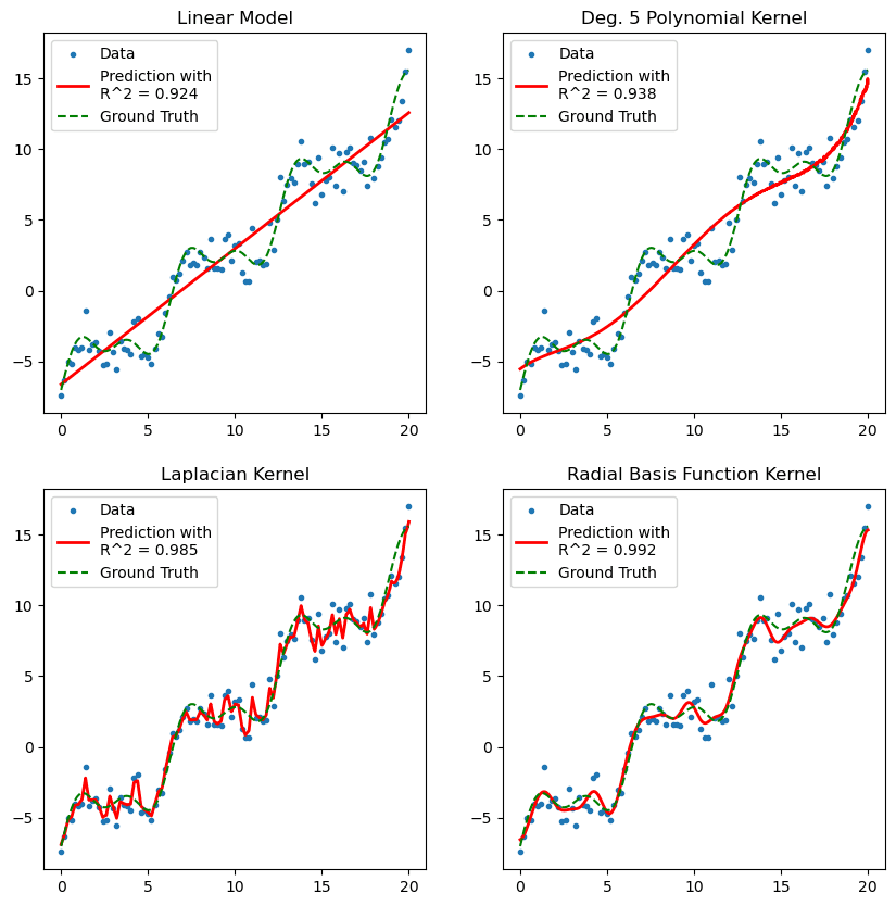
Figure 1. Diagram of various kernels used to fit data using the Kernel Ridge Regression model.
Back to our example
Recall our running dataset from the previous example.
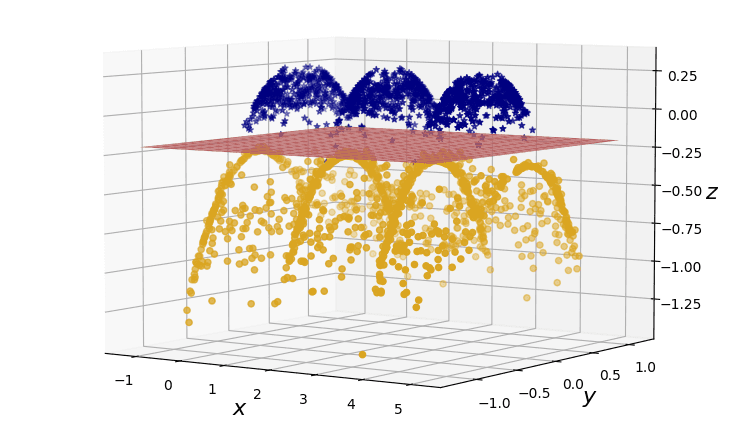
Figure 2. A dataset projection to produce linearly seperable data.
The kernel that makes the projection from 2D to 3D in our two-dimensional problem would correspond to the product
This is the sum of a linear kernel, , and the norm of a non-linear mapping .
Remember, in machine learning, it is not the task of the user to derive these projections by hand. This is the part where the algorithm itself will find the optimal projection.