In this tutorial, we shall take our first step away from linear models, and begin identifying more complex, non-linear patterns in real-world data. We begin with an example problem which is not linearly solvable in two dimensions, and show that a solution presents itself in higher dimensions. This lends itself to the idea of the kernel trick, a clever mathematical method which enables building non-linear models with linear methods.
- Identifying linearly seperable data
- The difference between parametric and non-parametric models
- The importance of model flexibility to identify unforeseen feeatures
- Understanding the benefit of projecting features into higher dimensions
Pushing data into new dimensions
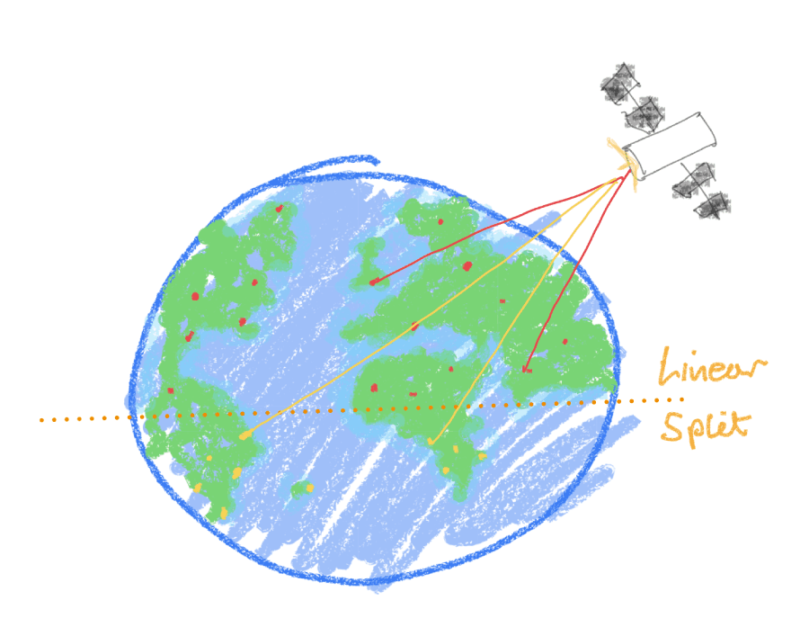
Figure 1. Data points recorded in the north and southern hemisphere are linearly, split by the equator.
Does your data split linearly? Whether your task is classification or regression, your key task as a data scientist is to make predictions from the patterns in your dataset. If these patterns can be separated by straight lines, we can use a linear regression model to make predictions of the form
where the features contribute to the outcome in proportion to the constants , which we optimise in advance: this is the ultimate interpretable model as the indicates relevance of the -th feature.
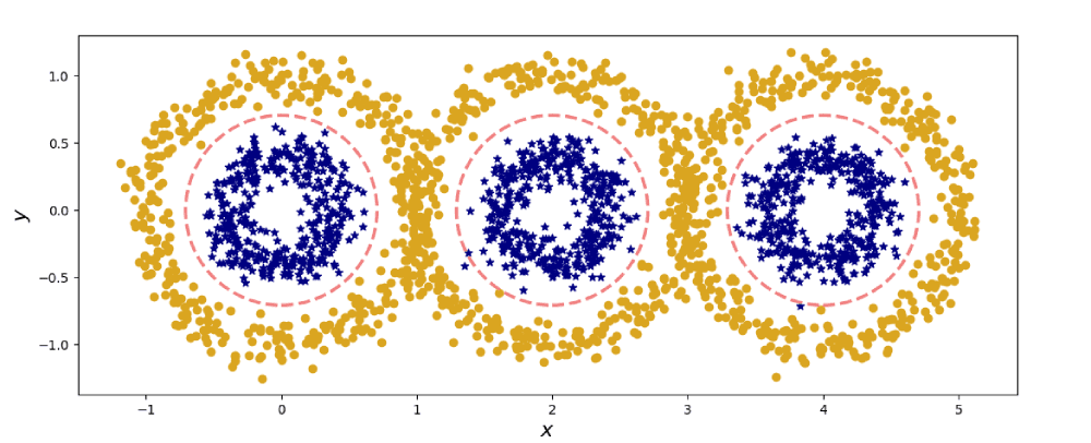
Figure 2. Non-linear data in two dimensions.
However, life is rarely so straight forward. For instance, how would you analyse the data in Fig. 2? By-eye inspection shows us that we could chalk out the blue centres of the three gold blobs. But without our human know-how, how might a machine identify these rings within rings?
💡 Answer: Project into new dimensions.
All a matter of perspective
What may look like a ring to us, may appear as flat surface (a linear model) in 3D. But how do we get there? Let's go ahead and project onto a third dimension. To do this, let's systematically examine the patterns in the two-dimensional data. Along the horizontal axis, we see three peaks of blue amidst the troughs of gold; a periodic structure of the form . Along the vertical axis we observe a central peak of blue with decaying gold, similar to the quadratic function . So let us plot a projection map , from two dimensions into three, given by
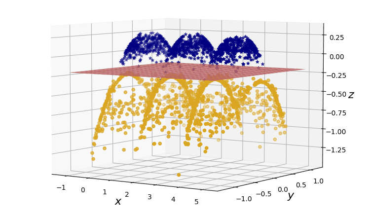
Figure 3. Linearly-separable data in three dimensions.
Success! Stretching our two-dimensional dataset into this third dimension allows us to drive a linear plane straight through the blue and golden data points.
In machine learning we ask the computer to do the heavy lifting. In fact, for subtle pattern recognition tasks, the whole point is that a sophisticated model will very often be able to disect data better than humans. The art is in choosing the correct model; such as a kernel method.