Let's consider our data problem more generally. If we have a $D$-dimensional dataset $\mathbf{x} = (x_1,\ldots,x_D)\in \mathbb{R}^D$, we can to stretch it into a much higher number of dimensions $H\gg D$ so that the problem is more easily separable. This leaves us defficit in on two accounts:

• Tractability: as the number of dimensions increases, fitting models involve learning more parameters which may require vast amounts of computational resources.
• Explainability: with large amounts of dimensions $D$, it can be difficult to systematically decide how to project the features into even higher dimensions $H$.

Let's recount the solution to the least squares regression problem. But first of all, let's postulate a projection of our data $\boldsymbol{\phi} = \mathbf{\phi}(x_1, \ldots, x_D)\in\mathbb{R}^H$ into a higher dimensional space. Our linear model from before now reads as $f = \sum_{i=1}^{H}\phi_{i}\beta_{i}$ for a larger vector of parameters. The analytical solution to minimising the squares of parameters $|\sum_i\beta_i^2|$ does not depend on the projected features $\phi_i$ themselves, but the products between them (written as $\phi_i\times\phi_j'$ for any two $\boldsymbol{\phi}, \boldsymbol{\phi}'$).

The so-called kernel trick is to recognise these products as the outputs of special types of functions, called "kernels". The outputs will depend only on pairs of input data features $\mathbf{x}, \mathbf{x}'$:

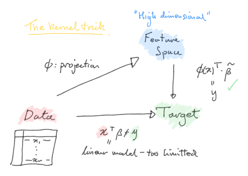
Diagram to show the shortcut taken by the kernel trick.

Making careful choices of the kernel function $k$ avoids need for ever explicitly writing down $\boldsymbol{\phi}$, which for very large $H$ may be very inconvenient to do.

The higher projection dimension is always treated theoretically, and with the kernel trick we can evaluate models in the projected space via scalar products. In this way, we can formalise the method to treat models in infinite dimensional spaces $H=\infty$ without having to explicitly compute in these spaces.