- Applying the Kernel Ridge Regression model with scikit-learn
- Exploring hyperparameters and kernel choices
- Visualising output
In this video, we'll get stuck straight in to our problem: predicting the compressive strength of concrete from a few easy to measure variables. This is an end-to-end implementation of kernel ridge regression that you'll need when deploying in the wild.
Inspect the data
Loading the data and inspecting the columns, we print out the following table:
Target:  Concrete compressive strength(MPa, megapascals)
Features:  Index(['Cement (component 1)(kg in a m^3 mixture)',
       'Blast Furnace Slag (component 2)(kg in a m^3 mixture)',
       'Fly Ash (component 3)(kg in a m^3 mixture)',
       'Water  (component 4)(kg in a m^3 mixture)',
       'Superplasticizer (component 5)(kg in a m^3 mixture)',
       'Coarse Aggregate  (component 6)(kg in a m^3 mixture)',
       'Fine Aggregate (component 7)(kg in a m^3 mixture)', 'Age (day)'],
      dtype='object')
X shape:  (1030, 8)
y shape:  (1030, 1)
This tells us that there are 8 input features from which we want to predict a single target: the compressive strength of concrete.
Preprocessing
We'll need to scale and centre the data set so it is clean for machine learning. We'll also split it into training and test sets.
from sklearn.model_selection import train_test_split
from sklearn.preprocessing import StandardScaler


X_train, X_test, y_train, y_test = train_test_split(
    X, y, test_size=0.2, random_state=31)

print('X_train shape: ', X_train.shape)
print('X_test shape: ', X_test.shape)
print('y_train shape: ', y_train.shape)
print('y_test shape: ', y_test.shape)

scaler = StandardScaler()
scaler.fit(X_train)

# Transform both X matrices with these values
X_train = scaler.transform(X_train)
X_test = scaler.transform(X_test)
Try a baseline linear model
So that we can benchmark any improvement, we'll first try a linear model.
from sklearn.linear_model import LinearRegression

# Fit a linear model
linear_model = LinearRegression()
linear_model.fit(X_train, y_train)
The results aren't aweful, but indicate there is much more to be done with an score of 0.58.
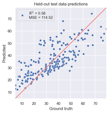
Figure 1. A plot of the predictions vs. the ground truth for a baseline linear fit.
The Kernel Ridge Regressor
Our assumption is that a non-parametric model can learn the non-linear behaviour found in the residuals of the linear model. This is where subtle feature extraction can improve the fit.
from sklearn.kernel_ridge import KernelRidge

# Fit a KRR model
krr= KernelRidge(kernel='polynomial', degree=4, alpha=1.0)
krr.fit(X_train, y_train)


y_pred_linear = linear_model.predict(X_test)
y_pred_poly = krr.predict(X_test)
The results give us a far improved model.
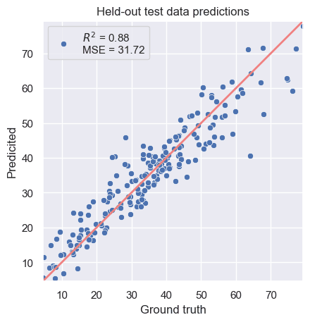
Figure 2. Kernel Ridge Regression solution.
Tune the model over parameter space
In the implementation, we specified a number of hyper parameters kernel, degree, alpha. To ensure that we make the best possible choice, we can automate a search through the options and assess the outcome with K-fold cross validation.
First of all, let's specify the parameters that we shall search through.
param_grid = [
    {'degree': [2, 3, 4, 5, 6],
     'alpha': [1e-1, 1.0, 10],
     'kernel': ['polynomial'],
    },
    {'gamma': [1e-2, 1e-1, 1, 10],
     'alpha': [1e-1, 1.0, 10],
     'kernel': ['rbf'],
    },
]
Then we can perform the grid search.
from sklearn.model_selection import GridSearchCV, RepeatedStratifiedKFold

krr = KernelRidge()
cv = RepeatedStratifiedKFold(n_splits=10, n_repeats=10, random_state=0)
search = GridSearchCV(
    estimator=krr, param_grid=param_grid,
)
search.fit(X_train, y_train)
This object now contains a search.best_estimator_ which we can compute the score on and recall the kernel. In fact, if we want to call upon more outputs of the search, we can return the values as a pandas.dataframe:
df = pd.DataFrame(search.cv_results_)
df[df['param_kernel'] == 'polynomial'][df['param_alpha'] == 0.1]
Which gives a complete overview of the K-fold cross validation statistics to report upon. Don't forget the df.to_markdown() method!
| mean_fit_time | std_fit_time | mean_score_time | std_score_time | param_alpha | param_degree | param_kernel | param_gamma | params | split0_test_score | split1_test_score | split2_test_score | split3_test_score | split4_test_score | mean_test_score | std_test_score | rank_test_score | |
|---|---|---|---|---|---|---|---|---|---|---|---|---|---|---|---|---|---|
| 0 | 0.313852 | 0.154708 | 0.11445 | 0.0619005 | 0.1 | 2 | polynomial | nan | {'alpha': 0.1, 'degree': 2, 'kernel': 'polynomial'} | 0.768445 | 0.799914 | 0.799908 | 0.742548 | 0.809902 | 0.784143 | 0.0250491 | 12 |
| 1 | 0.323135 | 0.0222913 | 0.0726411 | 0.0193653 | 0.1 | 3 | polynomial | nan | {'alpha': 0.1, 'degree': 3, 'kernel': 'polynomial'} | 0.864129 | 0.895091 | 0.874832 | 0.841756 | 0.878514 | 0.870864 | 0.0176288 | 3 |
| 2 | 0.342396 | 0.0471995 | 0.0740518 | 0.0387501 | 0.1 | 4 | polynomial | nan | {'alpha': 0.1, 'degree': 4, 'kernel': 'polynomial'} | 0.874275 | 0.899858 | 0.913486 | 0.777022 | 0.875907 | 0.868109 | 0.0478807 | 4 |
| 3 | 0.32883 | 0.0436676 | 0.056971 | 0.0127754 | 0.1 | 5 | polynomial | nan | {'alpha': 0.1, 'degree': 5, 'kernel': 'polynomial'} | 0.840566 | 0.784525 | 0.686616 | 0.673168 | 0.698032 | 0.736581 | 0.0649849 | 17 |
| 4 | 0.305537 | 0.00571628 | 0.076536 | 0.0288526 | 0.1 | 6 | polynomial | nan | {'alpha': 0.1, 'degree': 6, 'kernel': 'polynomial'} | 0.792378 | 0.663244 | -0.0384043 | 0.462756 | 0.664408 | 0.508876 | 0.29327 | 19 |