In this code walk-through, we explore the algorithm for decision tree learning using the scikit-learn implementation. Experimenting on a visual classification problem, we explore how to interpret the models results to explain the predictions.

For this example, we are leaning into our favourite 2D demonstrator: the blobs. Let's begin by importing the data.

def blobs(num_samples, std_dev, seed):
    """Generate two 2D normal distributions in the NE and SW quadrants."""
    cov = np.asarray([[std_dev, 0], [0, std_dev]])
    mean_ne = np.asarray([2., 2.5])
    mean_se = np.asarray([2.5, 1.5])
    mean_sw = np.asarray([1.5, 1.5])
    np.random.seed(seed)
    ne = np.random.multivariate_normal(mean=mean_ne, cov=cov, size=num_samples)
    se = np.random.multivariate_normal(mean=mean_se, cov=cov, size=num_samples)
    sw = np.random.multivariate_normal(mean=mean_sw, cov=cov, size=num_samples)
    return ne, se, sw

As before, sampling from this data generator gives us the following dataset:

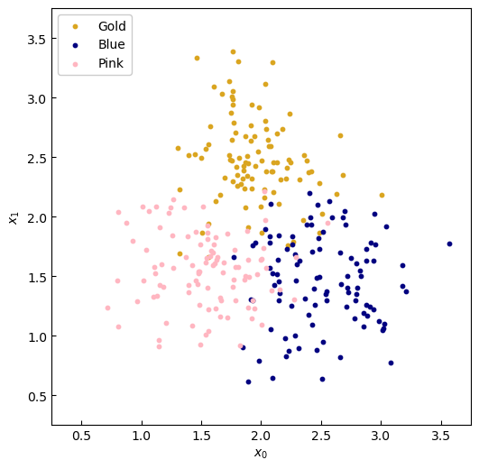
Figure 1. Sample data.

Let's try and solve a more dificult problem--a classification problem--using the power of machine learning to optimise our decision tree splits. This shall lead us to an algorithm, and hence a model, that can be deployed on general datasets.

For this exampole, here's the data: We collect 300 samples, split equally amongst three generic classes: 'Gold', 'Blue' and 'Pink'.

Our next step is to preprocess the data in the scikit-learn format:

from sklearn.utils import shuffle
from sklearn.model_selection import train_test_split

NUM_SAMPLES = 100
NOISE = 0.12
ne, se, sw = blobs(NUM_SAMPLES, NOISE, 31)

# Organise the data
X = np.concatenate((ne, se, sw), axis=0)
y = np.asarray(len(ne)*[-1,] + len(se)*[1,] + len(sw)*[0,])

# Randomly order the data, for good measure
X_train, y_train = shuffle(X, y, random_state=31)

Then we are ready to train our decision tree.

from sklearn.tree import DecisionTreeClassifier

MAX_LEAF_NODES = 3

model = DecisionTreeClassifier(
    random_state=SEED, max_leaf_nodes=MAX_LEAF_NODES,
)
model.fit(X_train, y_train)

Of upmost importantly, we wish to interrogate and interpret the model. The tree structure lends itself to this analysis. To print out the graph of the tree we use the export_text utility.

from sklearn.tree import export_text

read_out = export_text(model)
print(read_out)

|--- feature_1 <= 2.15
|   |--- feature_0 <= 2.06
|   |   |--- class: 0
|   |--- feature_0 >  2.06
|   |   |--- class: 1
|--- feature_1 >  2.15
|   |--- class: -1

To visualise this same graph we can use graphviz.

import graphviz
from sklearn.tree import export_graphviz

gv = export_graphviz(model, out_file=None)
graph = graphviz.Source(gv)
graph.render('images1/blobs-graph3', format='png')
graph

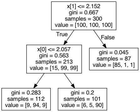
Figure 2. Output of `graphviz`.

Finally, to demostrace the decision boundaries, we plot the contours of the model.predict function.

x = np.linspace(AX_MIN, AX_MAX, 1000)
y = np.linspace(AX_MIN, AX_MAX, 1000)
xx, yy = np.meshgrid(x, y)

# Predict contours
f = model.predict(np.c_[xx.ravel(), yy.ravel()])
ff = f.reshape(xx.shape)

from matplotlib import cm

# x-axis
x0 = np.linspace(LINE_MIN, LINE_MAX, 1000)

# Plot data and ground truth
fig, ax = plt.subplots(1, 1, figsize=[6, 6])
plt.subplots_adjust(wspace=SPACE, hspace=SPACE)

# Axes
ax.tick_params(direction='in')
ax.set_xlim(AX_MIN, AX_MAX)
ax.set_ylim(AX_MIN, AX_MAX)
# ax.get_xaxis().set_visible(False)
# ax.get_yaxis().set_visible(False)
ax.set_xlabel('$x_0$')
ax.set_ylabel('$x_1$')

# Plot data
gold = ax.scatter(ne[:, 0], ne[:, 1], s=10, color='goldenrod')
blue = ax.scatter(se[:, 0], se[:, 1], s=10, color='navy')
pink = ax.scatter(sw[:, 0], sw[:, 1], s=10, color='lightpink')
# gt, = ax.plot(x0, -x0 + 4, color='lightcoral', linestyle='--', linewidth=2)

# Plot contour of predictive model
ax.contourf(
    xx, yy, ff, cmap=cm.get_cmap("magma_r"), alpha=0.5, linestyles=["-"],
)

ax.set_title(
    f'Decision tree of depth {model.get_depth()} '
    f'with {model.tree_.node_count} nodes')

ax.legend(
    [gold, blue, pink],
    ['Gold', 'Blue', 'Pink'],
    loc='upper left',
    framealpha=1.,
)
plt.show()

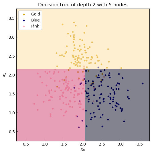
Figure 3. Coutours of the decision tree predictor.