Regression can be dealt with in a very similar fashion, by averaging output predicitons over discrete intervals. This has pros and cons. A pro is that it is simple, cheap and effective. A con is that you are returned with a highly discontinuous function which is prone to over fitting.

In this example, we are going off peast with a bespoke continuous function which we shall sample 50 times with Gaussian noise.

def sigmoid(x):
    return 1/(1 + np.exp(-x))

def demo(x):
    return sigmoid(x - 20) + 0.5 * sigmoid(10-x)

# Demo problem
NUM_SAMPLES = 50
NOISE = 0.07

np.random.seed(31)

X_true = np.linspace(0, 30, 1000)
y_true = demo(X_true)

X_train = np.linspace(0, 30, NUM_SAMPLES).reshape(-1, 1)
y_train = demo(X_train) + np.random.normal(0, NOISE, X_train.shape)

print('x shape: ', X_train.shape)
print('y shape: ', y_train.shape)

gt, = plt.plot(X_true, y_true, 'g', linewidth=2)
scat = plt.scatter(X_train, y_train, marker='.')
plt.legend([scat, gt], ['Data', 'Ground Truth'])
plt.show()

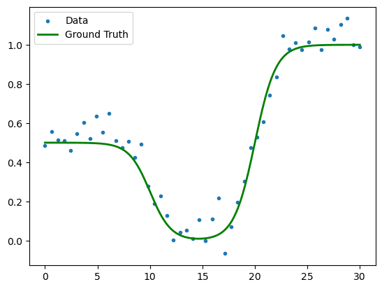
Figure 1. Sample regression data with three plateaux.

We have chosen this function to exhibit the nature of how a decision tree fits to continuous data: in summary, discretely. We are hoping our model shall find each of the three flat parts. The we shall extend its freedom and inspect the outcome when it over fits.

Training the Regressor

Just as before we use the scikit-learn implementatino alongside the graphviz package to visualise the tree.

import graphviz
from sklearn.tree import DecisionTreeRegressor, export_graphviz

model = DecisionTreeRegressor(random_state=31, max_depth=10)
model.fit(X_train, y_train)

gv = export_graphviz(model, out_file=None)
graph = graphviz.Source(gv)
graph

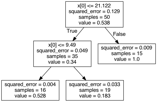
Figure 2. A graph of the tree regressor.

In the tree diagram we can see that the data still has many samples on each (terminal) leaf node and has significantly reduced the error at each stage. A good sign that we are well approximating the dataset.

To plot the output, we inspect the prediction function alongside the slitting thresholds.

y_pred = model.predict(X_true.reshape(-1, 1))
gt, = plt.plot(X_true, y_true, 'g', linewidth=2)
pred, = plt.plot(X_true, y_pred, '--r', linewidth=1.5)
scat = plt.scatter(X_train, y_train, marker='.')
split = plt.axvline(
    x=model.tree_.threshold[0] - 0.03, color='peru', linewidth=2.5, linestyle='-'
)
plt.axvline(
    x=model.tree_.threshold[1], color='peru', linewidth=2.5, linestyle='-'
)
plt.legend(
    [scat, gt, pred],
    ['Data', 'Ground Truth', 'Prediction'],
)
plt.show()

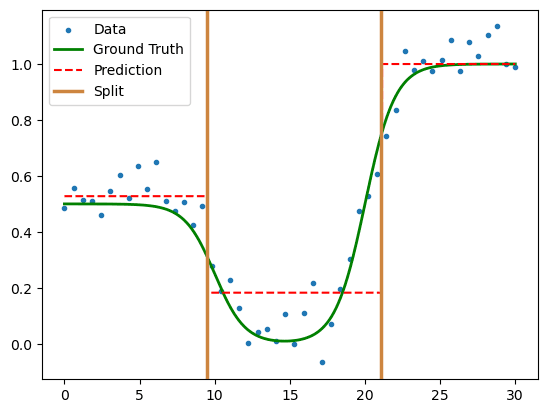
Figure 3. Output prediction of a 3-leaf node regressor.

Validation

We measure the success with the R2-score between predictions and ground truth.

from sklearn.metrics import r2_score

np.random.seed(33)
X_test = np.linspace(0, 30, NUM_SAMPLES).reshape(-1, 1)
y_test = demo(X_test) + np.random.normal(0, NOISE, X_test.shape)


r2_test = r2_score(y_test, model.predict(X_test))
r2_train = r2_score(y_train, model.predict(X_train))

print(f'R2 score (train): {r2_train:.2f}')
print(f'R2 score (test): {r2_test:.2f}')

R2 score (train): 0.88
R2 score (test): 0.87

We observe very close values. There is significant correlation between the output and input, but as the value is held on the test set, we don't expect overfitting.

Now let's lift the limit on the tree's predictive power and allow

max_depth = 10

with no restriction on max_leaf_nodes. From the output, it is clear the model has over fit.

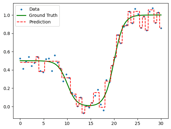
Figure 4. An over-fit regression tree.

Each training point now has its own interval especially for it. But in high dimensions, it might be dificult to plot data in this way. We can instead detect overfitting by considering the R2 metric from before.

r2_test = r2_score(y_test, model.predict(X_test))
r2_train = r2_score(y_train, model.predict(X_train))

R2 score (train): 1.00
R2 score (test): 0.93

Whilst we have had increase in on the test set, from 0.87 to 0.93, the training data is now perfectly correlated with the model predictions.