In this tutorial, we introduce the basis for a new family of models called tree-based algorithms. This will be our first encounter with a 'deep' model, but one whose depth may be meaningfully interpreted. Decision trees on their own are vulnerable, with risk to over fitting. But they are important modules in state-of-the-art algorithms such as the random forest.

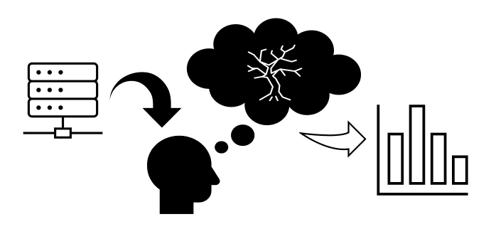
Figure 1. We form decision trees in our own thought processes to make decisions based on data or the environment.

Decision trees are supervised learning algorithms and can be used to solve both regression and classification tasks. They are deterministic: once a tree is trained, they follow a fixed set of rules to generate predictions. In fact, you probably already use such rules on a daily basis. So let's walk through the fundamental concept with an example.

Here's your dilemma: It's 8pm. You are at home, in your onesie, finishing an important assignment for the morning. You're 80% finished, but there is no room for error on the report. Then you receive a call: "Hey, we're all here. Come and join us at the pub." :beers:

Should you stay or should you go? Let's try to deconstruct the problem. To start, we have a set of input data:

We want to let these data govern an outcome $y \in \{\text{stay}, \text{ go}\}$. So let's build a model that sifts the input into one of these outcomes by asking ourselves some leading questions:

1. Is it late?
2. Is the work nearly finished?
3. Too comfy?

We can answer these questions, in some order, and decide how important the features of $\mathbf{x}$ are to the outcome. In Fig. 2, we build a tree model that results in the outcome $y$ telling us to STAY! This may not be the outcome we were hoping for. But the building blocks of the model allow us to arrive at this decision in a systematic way, by asking binary questions of our input vector $\mathbf{x}$. Once a question is asked, the problem is split into two. Asking sufficiently many questions splits the data such that we narrow down to an outcome.

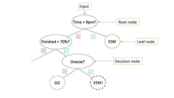
Figure 2. A human-constructed decision tree to help make the decision between staying to work or go to the pub. The green boxes indicate standard terminology of elements in the diagram (see below). The dashed red node indicates the final decision reached by following the tree.

Is this a good predictive model?

Do not be deceived: no machine learning has occurred in the construction of Fig. 2. Our goal is to write an algorithm that finds the best possible tree structure given a set of known data $\rightarrow$ outcome pairs $(\mathbf{x}_n, y_n)$. We can we improve tree models in a couple of ways:

• Question order: Each question is querying a different feature in $\mathbf{x}$. By choosing the feature with maximum impact first, we may reach a decision more quickly. For example, perhaps the question to stay or go is always simply determined by one factor alone.

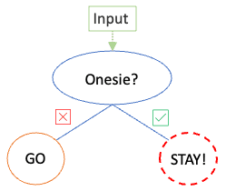
Figure. 3. A refined tree with the same predicitive power with just one node.

• Threshold adjustment: In this model our data is not solely categorical (e.g. are you wearing a onesie) but contains continuous values (e.g. time of day). We should split continuous variables at particular thresholds that best split the data.

Terminology

Even though the model in Fig. 2. may be imperfect, it showcases some terminology used to describe the components of decision trees:

• Root node This is where it all starts: the first node of the tree is where the data enters and we ask our first question.

• Decision Node A decision node is one at which a splitting occurs. At this point we nominate a data feature and a threshold value with which to split the data.

• Leaf Node (a.k.a. terminal node) A leaf node is defined where the data has been optimally split. Either each data sample had been assigned its correct class, or we have engineered the tree to always terminate at a specified leaf node. (The latter could be achieved by fixing the maximum depth we are willing to go to.)

• Pruning In typical models, there may be multiple paths that arrive at a similar outcome. Removing intermediate decision nodes, either pre- or post-optimisation, will reduce overfitting and improve generalisability (to new unseen data).