In this tutorial, we introduce the basis for a new family of models called tree-based algorithms. This will be our first encounter with a 'deep' model, but one whose depth may be meaningfully interpreted. Decision trees on their own are vulnerable, with risk to over fitting. But they are important modules in state-of-the-art algorithms such as the random forest.
- Examine the decision tree algorithm for machine-trained trees.
- Demonstrate its functiuonality on a classification example.
- Examine ways to quantify success of the algorithm during training.
- Introduce the notion of decision trees for regression problems.
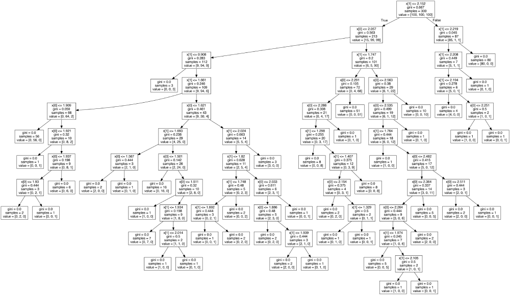
Figure 1. Following the decision trail of a machine designed tree.
Machines that learn trees
Let's try and solve a more dificult problem--a classification problem--using the power of machine learning to optimise our decision tree splits. This shall lead us to an algorithm, and hence a model, that can be deployed on general datasets.
For this example, here's the data: We collect 300 samples, split equally amongst three generic classes: 'Gold', 'Blue' and 'Pink'.
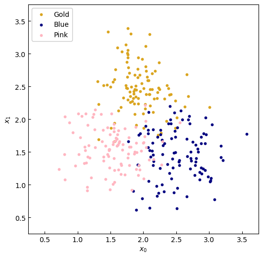
Figure 2. Sample data.
The classes are gathered in clusters, albeit with some overlap at the boundaries. A good machine learning model would disregard this as noise, and still produce the overall trend in the data. Our data points come in the form along the two axes of the graph. To fit a decision tree we follow the following steps:
- Which feature, or , maximises the split in the data.
- What is the cut-off in that feature which maximises the data split.
Applying this reasoning twice, we obtain the following graph.
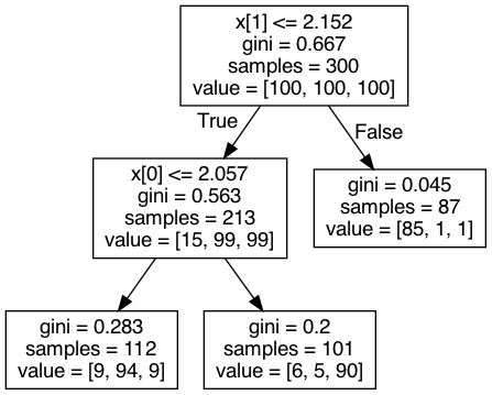
Figure 3. Output of the Decision Tree Classifier.
The top node--the 'root node'--indicates to first split the at . This choice determines the greatest split of the data, with 87 having and the remaining larger. The next best splitting of the data is to look at the node with samples and split the variable at . Let us visualise these two decisions as lines splitting the data.
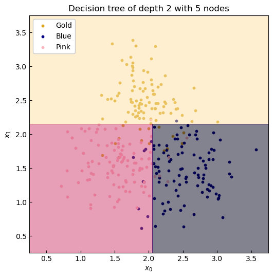
Figure 4. Coutours of the decision tree predictor.
Intuitively, this seems like a good fit. We have constructed a tree with 5 nodes, two decision nodes and three leaf nodes, which is just two layers deep. So let's measure the accuracy of this model on both the training set and the held-out test set.
| Depth 2 | Accuracy |
|---|---|
| Training set | 88.7% |
| Test set | 89.6% |
😋 This method of optimisation is known as greedy optimisation: at a given node, we do not worry about the best answer with respect to the whole tree, simply how best can we split the data set at that point. This is a short-cutting technique and the benefit in speed is typically exponentially greater than costs in accuracy.
The error recorded here is dependent on the inherent noise in the data. Visually, we can see a trend of three clusters, so this model is the correct choice. But what were to happen if we allowed tree to split further until the entire training set was correctly classified?
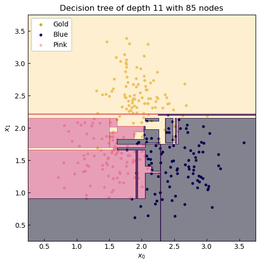
Figure 5. Over fitting can kreep in when hyperparameters permit too much flexibility.
Now we have begun to 'overfit'. Here we left the tree to classify each data point perfectly, so that accuracy would be 100% on the training set. But by inspection, we can't expect this tree to describe unseen data--and this point is demonstrated when the performance is evaluated on the testing set.
| Depth 10 | Accuracy |
|---|---|
| Training set | 100.0% |
| Test set | 83.3% |
What can we conclude? Decision trees are powerful tools for classification, but without user interference, as we did by limiting the model freedom (the depth), they run the risk of over-fitting to training data (and so produces a model which is not useful). Hang on to your seats as we visualise the graph of the tree in the headline Fig. 1.
What mechanisms can we use to automatically optimise these trees? Our objective is to maximise the number of samples into their correct classes. For classification, this could be achieved with:
- Gini impurity: a measure of how often a randomly chosen data point would be misclassified by a new splitting.
- Entropy: a measure of chaos, which in this case penalises all classes being equally well represented in a splitting.
Or in the case of regression:
- The Mean Squared Error: given that in regression problems we have no classes, we penalise splittings in which the mean of the data in each split generates the most absolute error with the ground truth.